"Scale space" is a term from Computer Vision, see Lindeberg (1994) Scale Space Theory in Computer Vision, that means a family of Gaussian kernel smooths indexed by the bandwidth. This has a number of interesting implications for both the theory and practice of smoothing in statistics, as discussed in Chaudhuri and Marron (1997, PDF version (862 KB) | Postscript Version (4.64 MB) ). An application to finding statistically significant structure in univariate smoothing, called SiZer was developed in: is given in Chaudhuri and Marron (1999, 2,334k postscript file | 366k GNU Zipped (.gz) | 442k Compressed (.Z) ).
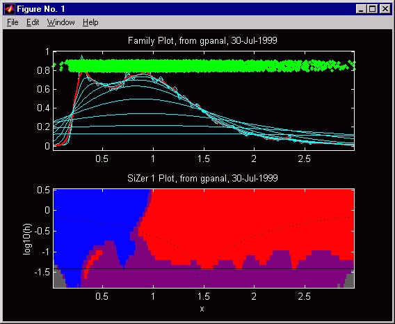
Here is an example illustrating the use of SiZer, for the income data,
see e.g. Marron and Schmitz(1992) Econometric Theory, 8, 476-488.
for more about these data, including another way seeing that there are
two modes.
This newer work studies related ideas in the context
of 2-d images. There were two major hurdles. First the concept
of "slope" is more complicated in 2-d, and thus required new ways of thinking
about its "statistical significance". Second the higher dimensionality
required a new visual paradigm. This was done via movies which "morph
through the family of smooths", with bandwidth (i.e. scale) represented
by time.
3a. Image Analysis
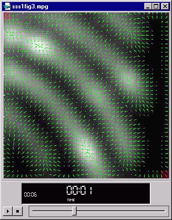
Full details of the SSS in the context of image analysis are developed in Godtliebsen, Marron and Chaudhuri (1999a) [ PDF version (701 KB) | Postscript Version (3.61 MB) ]. The basis is a family of Gaussian kernel smooths, indexed by the bandwidth, shown as a movie of gray level plots. This is seen for some gamma camera data in this movie.
The simplest approach to understanding statistical
significance of features in each smooth is based on gradients. When
the gradient is significantly different from 0 (i.e. there is some "statistically
significant slope"), and arrow is drawn in the gradient direction.
Here is one frame of this movie, representing one scale, i.e. level of
smoothing.
(Caution: this is only a "screen shot", so the buttons don't work.
Click here
to see this movie)
The arrows show that the diagonal ridges are "really there", as are
the faintly brighter spots at a few locations, in particular the barely
bright spot near the center of the image. This movie version shows
how this evolves over the full range of smoothing scales.
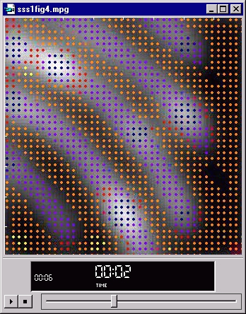
Another approach is based on significant curvature.
See the paper [ PDF
version (701 KB) | Postscript
Version (3.61 MB) ] for details, but the main idea is that colored
dots reflect different types of significant curvature, as shown here.
(Caution: this is only a "screen shot", so the buttons don't work.
Click here
to see this movie)
These highlight the ridges and valleys in a different way, and again
show that the bright spots are "really there". Since different features
show up at different levels of resolution, it is worth looking at the full
movie
.
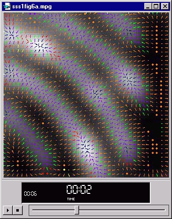
The arrow and dot visualizations can be combined
to give:
(Caution: this is only a "screen shot", so the buttons don't work.
Click here
to see this movie)
A weakness of the above visualizations is the "raster
effect" caused by the symbols lying on a rectangular grid. This is
distinctly not "rotation invariant". Current thought on the presentation
of vector fields of directional data is that a better presentation device
is "streamlines", which are continuous lines that follow the gradient direction.
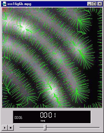
(Caution: this is only a "screen shot", so the buttons don't work.
Click here
to see this movie)
This is a different way of seeing the significance of the same features.
Again the movie version is well worthwhile.
Many more examples that illustrate the usefulness of this method, and also that test it in various ways, may be found in the paper [ PDF version (701 KB) | Postscript Version (3.61 MB) ].
General purpose Matlab software, that made
these movies, and also can be easily used on other data sets is available
at http://www.unc.edu/depts/statistics/postscript/papers/marron/SSS_software/.
The whole collection of files should be downloaded, e.g. to a single directory,
because many of them call each other. The Matlab subroutine conv2.m,
in the Signal Processing toolbox is required. The main call is to the subroutine
sss1.m. The Matlab command
">> help sss1" gives information
about how to use the various versions of SSS.
3b. Bivariate Density Estimation
The visualizations developed above have been adapted to density estimation, in Godtliebsen, Marron and Chaudhuri (1999b) [ PDF version (451 KB) | Postscript Version (2.02 MB) ].
An example illustrating this is the Melbourne Daily
Maximum Temperature Data, analyzed by Hyndman, Bashtannyk and Grunwald
(1996) Journal of Computational and Graphical Statistics, 5, 316-336.
Here is a "lag one scatterplot" of the data, where the x-axis represents
yesterday's maximum and the y-axis represents today's maximum.

Note there is an apparent ridge along the line y=x, which is
consistent with the idea of predicting today's max by using yesterday's
max. Less clear, but graphically presented by Hyndman, et. al., is
a "horizontal arm", near the line y=20.
Our SSS methodology not only shows that this arm is statistically significant, but also finds another vertical arm. Both arms have been explained by meteorologists via a continental warm air mass changing places with sea breezes.
This can be seen with any of our visual approaches:
Significant
Arrows
Significant
Dots
Significant
Arrows and Dots
Significant
Streamlines
Note that two arms show up at different times in the movies, i.e. at
different levels of resolutions, or different amounts of smoothing.
Perhaps the streamline view is best:


(Caution: these are only "screen shots", so the buttons don't work.
Click here
to see this movie)
As for the image version of SSS, more examples that illustrate the usefulness of this method, and also that test it in various ways, may be found in the paper [ PDF version (451 KB) | Postscript Version (2.02 MB) ]. For a detailed index of figures and movies in the paper, go here.
General purpose Matlab software (actually the same
subroutine), that made these movies, and also can be easily used on other
data sets is available at http://www.unc.edu/depts/statistics/postscript/papers/marron/SSS_software/.
The whole collection of files should be downloaded, e.g. to a single directory,
because many of them call each other. The Matlab subroutine conv2.m,
in the Signal Processing toolbox is required. The main call is to the subroutine
sss1.m. The Matlab command
">> help sss1" gives information
about how to use the various versions of SSS.
Back to Movies Table of Contents
Back to Marron's Home Page